Smaller Classes with Fewer Teachers

Identifying the costs of teacher misallocation in South Africa

Peter Courtney

Stellenbosch University & Tinbergen Institute
Slides: petercourtney.co.za

2026-03-01

PART I: THE PUZZLE

Learners per teacher on payroll: 32.5

Learners in the average classroom: 43.3

Schools employ enough teachers for classes of 32 but deliver classes of 43.

---

This gap costs R22.3 billion per year — 18% of the national teaching wage bill.

EMIS + LURITS administrative records, 2022–2024. N = 6,291 ordinary public primary schools. Author’s calculations.

TALK: I want to start with a simple puzzle. South African primary schools employ enough teachers for classes of 32 learners. But the average child sits in a class of 43. That is not a small gap. It represents R22.3 billion per year — about 18 per cent of everything the state spends on teacher salaries — in instructional capacity that is purchased but never reaches the classroom.

A Global Problem Hiding in Plain Sight

Country	Teachers per class	Class size	STR	Implication
Tanzania	2.50	82	45	60% of teacher time is non-contact
India (UP)	1.60	55	35	38% of teacher time is non-contact
Kenya	1.35	52	40	26% of teacher time is non-contact
South Africa	1.22	43	32.5	18% of teacher time is non-contact

Wherever I measure it, the gap between teachers employed and teachers deployed is massive.

Yet this margin is “remarkably understudied” — Bennell (2022). No country has administratively decomposed it until now.

Tanzania, Kenya, India: World Bank SDI reports and administrative data estimates. South Africa: author’s calculations.

TALK: And this is not a South African anomaly. Look at Tanzania: 2.5 teachers per class, yet class sizes above 80. That means 60 per cent of teacher time is non-contact. Kenya, India — the pattern repeats. Wherever we measure this gap between teachers employed and teachers actually deployed, it is enormous. And yet — this is the striking part — it is almost completely unstudied. Paul Bennell, reviewing the global evidence in 2022, called it “remarkably understudied.” No country has produced an administrative decomposition of where this slack comes from. This paper does that for the first time.

The Unmeasured Margin in Education Deployment

The Input Elasticity Puzzle

For decades, I have asked why hiring more teachers fails to improve learning.

My answer: Hiring does not shrink classes. New teachers are absorbed into organisational slack.

The Misallocation Literature

Research focuses on redistributing teachers between schools.

My finding: Within-school deployment slack dwarfs the potential gains from between-school spatial reallocation.

Both literatures assume teachers, once hired, are fully deployed. They are not.

TALK: Why should a room full of economists care about school class scheduling? Because it sits at the intersection of two of the largest literatures in education economics. First, the input elasticity puzzle. For four decades, since Hanushek 1986, the central puzzle has been: why doesn’t spending more on teachers improve learning? Hundreds of papers, thousands of citations. I provide a mechanical answer: new hires do not reduce class sizes. They expand the non-contact buffer. The money goes in, but instruction doesn’t come out. Second, the teacher misallocation literature. Walter 2020, Urquiola 2006 — the standard framework asks how to redistribute teachers across schools. But I show that the within-school deployment margin is far larger than the between-school margin. We have been trying to optimise the wrong thing. Both literatures share the same blind spot: they assume that once a teacher is hired and placed, she teaches. She doesn’t — not always.

The Absenteeism Narrative Is Wrong

The World Bank Service Delivery Indicators conflate two fundamentally different phenomena:

\[ \text{SDI "Class Absence"} = 1 - \frac{\text{Teachers in Classrooms}}{\text{Total Employed}} \]

44%

of SSA teachers “absent from class”

Bold et al. (2017)

48%

of those are at school but not scheduled

Scheduled non-contact time, not truancy

Administrative class scheduling reforms ≠ behavioural accountability interventions.

TALK: And then there is the dominant narrative in global education — teacher absenteeism. The World Bank’s SDI programme reports that 44 per cent of Sub-Saharan African teachers are “absent from class” at any given moment. Billions of dollars of policy attention have been directed at this number. But the SDI definition conflates two different things. When I reconstruct the full class schedule grid, I find that nearly half of those “absent” teachers are physically present at school. They are simply not scheduled to teach. This is not a teacher effort problem — it is a management deployment problem. And the policy response is completely different.

My Contribution: Four Gaps

1. Misallocation

Literature focuses on spatial reallocation between schools (Walter, 2020; Urquiola, 2006).

Finding: Within-school slack dwarfs potential spatial gains.

2. Management

Teachers-per-class ratio is “remarkably understudied” (Bennell, 2022).

Finding: First rigorous large-scale administrative decomposition of this wedge.

3. Input Elasticity

Why hiring fails to improve learning (Hanushek, 1986).

Finding: Hiring does not shrink classes; new teachers are absorbed into slack.

4. The Absenteeism Narrative

World Bank SDI focuses on “absent from class” (Bold et al., 2017).

Finding: 48% of “absent” teachers are at school, just not scheduled to teach.

TALK: To summarise: four literature gaps, four contributions. Misallocation — within-school dwarfs between-school. Management — the first administrative decomposition of the deployment wedge. Input elasticity — the mechanical reason why hiring fails. And the absenteeism narrative — half of the supposed absence is scheduled non-contact time, not truancy.

PART II: WHAT’S HAPPENING AND HOW BIG IS IT

The Data: Supply, Demand, and Outcomes

LURITS

Learner Unit Record Information and Tracking System

5.4 million individual learner-to-class assignment records

Reconstructs the complete class schedule for every school

→ Demand: who sits where

PERSAL

Personnel and Salary Administration System

Individual teacher records: school placement, transfers, departures

Tracks every teacher movement between schools

→ Supply: who teaches where

SBAs

School-Based Assessments

Standardised grade-level mathematics and reading scores

Measure learning value-added at school level

→ Production: what learners learn

Together: full supply of teachers, demand from learners, and the final production of learning outcomes.

LURITS + EMIS (2022–2024), PERSAL (2018–2024), SBA value-added (2018–2022). Not survey estimates — direct administrative records.

TALK: Let me describe the data, because it is unusual. I link three administrative systems. LURITS — 5.4 million individual records linking each learner to a specific class section. From this I reconstruct the complete class schedule for every school. PERSAL — the personnel system, tracking every teacher’s employment and movement. And School-Based Assessments — standardised scores for learning outcomes. Together, these give me the full supply-demand-production chain.

What I Constructed: The School Class Schedule

Scenario 1: Within-Grade Equalisation

Equal class sizes using original classes per grade

Grade	Learners	Classes	Class 1	Class 2	Class 3	Class 4	LECS
0	111	3	37	37	37		37.0
1	130	4	33	33	32	32	32.5
2	138	4	35	35	34	34	34.5
3	161	4	41	40	40	40	40.3
4	184	3	62	61	61		61.3
5	158	3	53	53	52		52.7
6	177	3	59	59	59		59.0
7	161	3	54	54	53		53.7
School	1,220	27					47.8

By reconstructing the class schedule, I can optimise class sizes using the existing teachers.

For example, I can equalise class sizes within grades to improve efficiency.

National average non-contact time: 18.2%. The same teachers could deliver classes of 33 instead of 40.

This grid is reconstructed from 5.4 million individual learner-to-class records.

Each cell is an observed assignment — not interpolated, not survey-based.

I observe this grid for every public primary school in the country.

School EMIS: 500294187. Actual class schedules reconstructed from LURITS + EMIS administrative records, 2022–2024.

TALK: This is the kind of data we work with. For every public primary school, we reconstruct the complete class schedule grid from administrative records. Each cell is an observed learner-to-class assignment. This allows us to see how classes are formed and where inefficiencies lie — such as unbalanced classes within the same grade. By optimising these allocations, we can find out what is possible. Nationally, the average non-contact time is 18 per cent. These are not estimates or imputations — these are direct administrative records covering 5.4 million individual learner assignments.

The Accounting Identity

\[\text{Student-Teacher Ratio} \;=\; \frac{\text{Class Size}}{\text{Teachers per Class}}\]

\[32.5 \;=\; \frac{43.3}{1.22}\]

STR = 32.5

Learners per teacher on payroll.

What the government tracks.

Class Size = 43.3

Learners each child actually sits with.

What children experience.

Teachers per Class = 1.22

The wedge between the two.

Where the leak is.

The same STR of 30 can mean classes of 30 (TCR = 1) or classes of 60 (TCR = 2).

EMIS + LURITS class schedule reconstruction, 2022–2024. 5.4 million individual learner-to-class assignment records.

TALK: Here is the accounting identity. Student-teacher ratio equals class size divided by teachers per class. When the government reports an STR of 32.5, that sounds manageable. But class size is 43.3. The ratio between them — teachers per class — is 1.22. That means 22 per cent more teacher-period slots than class slots. The surplus is not reducing class sizes; it is absorbed as non-contact time.

The Optimisation Algorithm

1. Objective
Minimise the enrolment-weighted average class size: \[\text{ECS} = \frac{1}{N} \sum_g \sum_{c \in g} \frac{n_{gc}^2}{n_g}\]

2. Constraints
- Teacher time: Each teacher has a fixed maximum number of periods. - Class coverage: Every scheduled class must have a teacher. - Integer assignment: Teachers cannot be fractionally assigned.

3. The Greedy Algorithm
The algorithm takes each school’s existing teachers and classrooms as fixed. It then greedily assigns available teacher periods to the largest unserved classes across all grades until all teacher time is exhausted.

🔍 Formal mathematical problem: B1

TALK: I formalise this with an algorithm. The objective is to minimise the enrolment-weighted average class size. The rules are strict: you only have the teachers currently on the payroll with their fixed number of periods, every single class needs a teacher, and teachers cannot be fractionally assigned. The greedy algorithm then takes the school’s existing teachers and classrooms, and greedily assigns teachers to the largest unserved classes until all teacher periods are exhausted. This finds the absolute minimum class size achievable with existing resources.

Where Does the Slack Live?

Observed class size: 43.3

→ Step 1: Balance class sizes within each grade (small gain)

→ Step 2: Reorganise classes across grades (moderate gain)

→ Step 3: Use idle classrooms (small gain)

→ Step 4: Use all available teacher time (massive gain)

Achievable class size with existing teachers: 35.2

Holding teacher numbers fixed, optimal deployment could reduce class sizes by 19%. Almost all of that gain comes from a single margin: putting existing teachers in front of classes.

TALK: Holding teacher numbers fixed — no new hiring — I ask: given the teachers you already have, what is the smallest class size you could achieve? The dominant margin is teacher utilisation. If you deployed existing teachers into existing time slots, class sizes fall from 43 to 35. A 19 per cent reduction with zero additional spending.

The Waterfall: Where the Gap Lives

Constrained optimisation on EMIS + LURITS class schedule reconstruction. N = 6,291 school-years, 2022–2024. Scenarios are nested (each adds one additional margin of adjustment).

🔍 Full scenario table: B1

TALK: Here is the national waterfall. Starting from observed class sizes of 43, I subtract the gains from each margin. Teacher utilisation — the gold bar — dwarfs everything else. Nearly all of the achievable gain comes from a single margin: the labour deployment margin.

The Numbers: Decomposing the Gap

Scenario	Constraint Relaxed	Margin	ECS	Cumulative
S0	Status quo (observed)	—	43.3	—
S1	Balance classes within grade	Within-school	42.8	−1.2%
S2	Optimise classes across grades	Within-school	42.3	−2.3%
S3	Activate idle classrooms	Within-school	38.9	−10.2%
S4	Full teacher utilisation	Within-school	35.2	−18.8%
S5	District-level teacher pooling	Between-school	32.8	−24.2%
S6	Province-level teacher pooling	Between-school	32.6	−24.6%

S4 alone delivers more than all other within-school margins combined.
S5–S6 (district and province pooling) add only 5.8 pp — yet all prior literature focused exclusively on this margin.

Source: Author’s constrained optimisation on EMIS + LURITS class schedule reconstruction. N = 6,291 schools, 2022–2024. Scenarios are nested.

TALK: Here are the exact numbers. S1 and S2 — class scheduling efficiency — deliver less than 2.5 per cent combined. S3 — idle classrooms — adds 8 per cent. S4 — teacher utilisation — delivers 18.8 per cent. That is the headline. But look at S5 and S6: district and province-level reallocation. These are the margins the entire misallocation literature has been focused on — Walter 2020, Fagernäs 2017, the whole spatial redistribution agenda. They add only 5.8 percentage points beyond what you can achieve within the school. The within-school labour margin is three times larger than the between-school spatial margin that has absorbed most of the research attention.

Efficiency Gaps Track Equity Gaps

• By Quintile
• By Race

Closing the deployment gap for the poorest would give them the same class sizes as the richest.

TALK: Who bears the cost? The poorest children. Q1 schools have baseline class sizes of 46; Q5 schools have 34. Deployment reform alone could cut Q1 from 46 to 38 without additional spending. The equity gap narrows dramatically under full utilisation.

PART III: WHY? THE NATURAL EXPERIMENT

Structural or Discretionary? The Test

“Structural”

The slack is forced by real structural constraints — teacher qualifications, building layout, integer problems in small schools.

If true: an external shock should reshuffle the constraints without systematically improving efficiency.

vs.

“Discretionary”

The slack is a legacy of past decisions that no one has revisited. Principals satisfice — the hassle of reorganising outweighs the perceived benefit.

If true: an external shock that forces reorganisation should make schools more efficient.

To distinguish, I need an external shock that forces schools to reorganise their class schedules.

TALK: We have established that 19 per cent of instructional capacity is idle. Why? One possibility: schools are stuck — real constraints force them into inefficient configurations. The other possibility: schools are discretionary — the current class schedule is a legacy of past decisions, and principals satisfice because reorganising is effortful and confrontational. To distinguish, I need an exogenous shock that forces reorganisation.

Why Demographic Shocks Force Reorganisation

Between-grade reallocation

Schools have a fixed number of teachers.

When a large cohort ages into a previously small grade, the school must create an additional class for that grade.

Creating a new class requires pulling a teacher from elsewhere in the class schedule.

This between-grade reallocation forces a school-wide reorganisation of the entire class schedule.

Why this matters for inference

The structural test: As lumpy cohorts move through a school, forced reconfiguration at the grade level should:

• ↑ inefficiency if constraints are structural — friction makes things worse
• ↓ inefficiency if inertia is the problem — forced action makes things better

TALK: Why would demographic shocks specifically test our hypothesis? Schools have a fixed number of teachers. When a large cohort ages in, the school must create an additional class. That requires pulling a teacher from another grade, which forces a school-wide reorganisation of the class schedule. If the configuration is just inertia — a legacy class schedule nobody bothered to revisit — then the shock should make things better, because the principal is forced past an inaction threshold and discovers a more efficient arrangement.

What Are Structural Frictions?

Examples of constraints

• Capital matching: Grade 1 rooms have small chairs and alphabet posters; they cannot easily become Grade 5 rooms.
• Teacher training: Foundation phase teachers cannot easily teach senior classes.
• Curriculum materials: Textbooks and assessment packs are locked to specific grades.

Implications for a lumpy cohort

When a demographic shock forces between-grade reallocation, these frictions bind:

• A room with the wrong furniture must be repurposed.
• A teacher with the wrong phase specialisation is pulled in.
• Reconfiguration is costly and constrained.

Result: Forced reorganisation under structural frictions should increase inefficiency.

TALK: What do we mean by structural frictions? Classrooms are not generic — a Grade 1 room has alphabet charts, small furniture, foundation phase materials. A teacher trained for Grade R cannot teach Grade 6. Curriculum packs and classroom layouts are grade-specific. If the existing configuration is genuinely constrained by these frictions, then a demographic shock that forces reorganisation should make things worse — you are disrupting a system that was already doing the best it could.

Seventeen Alternative Explanations: All Tested, All Rejected

#	Mechanism	Type
1	Grade-specific match capital	Structural
2	Qualification constraints	Structural
3	Period indivisibilities	Structural
4	Cross-phase synchronisation	Structural
5	Enrolment volatility buffering	Structural
6	Infrastructure constraints	Structural
7	Protected administrative roles	Structural
8	Health accommodations	Structural
9	Pull-out remediation programmes	Structural
10	Feeding-scheme logistics	Structural
11	SGB substitution	Structural
12	Standby rosters for absence	Structural
13	Data classification artefacts	Structural
14	Non-pecuniary compensation	Discretionary
15	Union bargaining	Discretionary
16	Discretionary specialisation	Discretionary
17	Institutional inertia	Discretionary

Key result: All structural predictions (β > 0) are rejected. The negative coefficients (β < 0) are consistent with policy equilibria where capacity exists but is withheld until external pressure forces action.

TALK: These are the seventeen alternative explanations I tested. The first five are genuinely structural — if they were binding, the demographic shock would make schools less efficient. All are rejected. The negative coefficients mean schools get more efficient when forced to reorganise. Rows 6-13 are operational or measurement explanations — none prevent reallocation when pressure arrives. The last four are policy equilibrium explanations — these are consistent with the data. The slack exists not because principals cannot reallocate, but because they face no pressure to do so.

How the Shock Works

When large and small birth cohorts are adjacent, the predicted age-progression creates sudden grade-composition shocks. These shocks are predictable from demographics but force real organisational responses.

Design feature: I use the demographic composition of the nearest 10 schools, excluding the focal school itself, so that a school’s own decisions never contaminate its instrument.

%%{init: {'theme': 'base', 'themeVariables': {'primaryColor': '#f5f5f5', 'primaryBorderColor': '#1a1a2e', 'lineColor': '#c8a96e', 'textColor': '#1a1a2e', 'fontSize': '17px', 'fontFamily': 'Inter,Helvetica,sans-serif'}, 'flowchart': {'htmlLabels': true, 'nodeSpacing': 30, 'rankSpacing': 55, 'curve': 'basis', 'padding': 20}}}%%
graph TD
    A["<b>Year <i>t</i></b><br>Small Grade 4 cohort<br>60 learners, 2 classes"]
    B["<b>Year <i>t+1</i></b><br>Grade 4 doubles<br>120 learners, 3 classes"]
    C["<b>Reconfiguration friction</b>"]
    D["Reassign a teacher"]
    E["Repurpose a room"]
    F["Rewrite the class schedule"]
    G["<b>School-wide reorganisation</b>"]

    A -->|"Large cohort ages in"| B
    B --> C
    C -->|"Staff"| D
    C -->|"Space"| E
    C -->|"Schedule"| F
    D --> G
    E --> G
    F --> G

    style A fill:#f5f5f5,stroke:#1a1a2e,stroke-width:2px
    style B fill:#f5f5f5,stroke:#c8a96e,stroke-width:2px
    style C fill:#c8a96e,stroke:#1a1a2e,stroke-width:2px,color:#1a1a2e
    style D fill:#f5f5f5,stroke:#1a1a2e,stroke-width:1px
    style E fill:#f5f5f5,stroke:#1a1a2e,stroke-width:1px
    style F fill:#f5f5f5,stroke:#1a1a2e,stroke-width:1px
    style G fill:#c8a96e,stroke:#1a1a2e,stroke-width:2px,color:#1a1a2e

TALK: Here is the mechanism. When a large cohort ages into a grade that previously had a small cohort, the school must create additional classes. That means pulling a teacher from somewhere else, repurposing a classroom that has the wrong materials and furniture, and rewriting the entire class schedule. This is a forced, school-wide reorganisation event. And the key design feature: I use the predicted demographics of the nearest 10 schools, excluding the focal school, so that the school’s own retention and admissions decisions never contaminate the instrument.

The Formal Specification

%%{init: {
  'theme': 'base',
  'themeVariables': {
    'primaryColor': '#f5f5f5',
    'primaryBorderColor': '#1a1a2e',
    'lineColor': '#8a8aaa',
    'textColor': '#1a1a2e',
    'fontSize': '16px',
    'fontFamily': 'Inter, Helvetica, sans-serif'
  },
  'flowchart': {
    'nodeSpacing': 50,
    'rankSpacing': 70,
    'curve': 'basis',
    'padding': 20,
    'wrappingWidth': 200,
    'htmlLabels': true
  }
}}%%
graph LR
    Z["<b>Z</b><br>LOO Neighbourhood<br>Demographics<br><i>(births 6–12 yrs ago)</i>"]
    X["<b>X</b><br>Grade Composition<br>Disruption"]
    Y["<b>Y</b><br>Allocative Efficiency<br><i>(TCR, ECS)</i>"]
    U["<b>U</b><br>Management quality,<br>unobserved constraints"]
    C["<b>Controls</b><br>ΔEnrolment, Year FE"]

    Z -->|"π (F = 39.8)"| X
    X -->|"β (causal)"| Y
    U -.->|"confounds"| X
    U -.->|"confounds"| Y
    C --> X
    C --> Y
    Z -.-x|"EXCLUDED<br>(LOO: own school<br>never enters Z)"| Y

    style Z fill:#f5f5f5,stroke:#c8a96e,stroke-width:2px
    style X fill:#f5f5f5,stroke:#1a1a2e,stroke-width:2px
    style Y fill:#f5f5f5,stroke:#1a1a2e,stroke-width:2px
    style U fill:#f5f5f5,stroke:#c8a96e,stroke-width:1px,stroke-dasharray: 5 5
    style C fill:#f5f5f5,stroke:#1a1a2e,stroke-width:1px
    
    linkStyle 6 stroke:#c0392b,stroke-width:2.5px

Leave-One-Out Cluster:

\[c(-i) = \{k{=}10 \text{ nearest schools to } i, \text{ excluding } i\}\]

Instrument:

\[Z_{c(-i),t} = \text{Predicted grade-composition disruption in } c(-i)\]

First stage:

\[\Delta X_{it} = \pi \cdot \Delta Z_{c(-i),t} + \gamma \cdot \Delta\text{Enrol}_{it} + \delta_t + \varepsilon_{it}\]

Second stage (2SLS):

\[\Delta Y_{it} = \beta \cdot \widehat{\Delta X}_{it} + \gamma \cdot \Delta\text{Enrol}_{it} + \delta_t + u_{it}\]

U (unobserved principal ability, preferences, constraints) confounds X and Y. The LOO demographic instrument Z breaks this confounding: births 6–12 years ago, in neighbouring schools, are orthogonal to current management choices.

TALK: The DAG makes the identification strategy transparent. The confounding problem is U — unobserved management quality. Good principals might simultaneously choose better grade configurations and run more efficient class schedules. The instrument Z breaks this: it is constructed from births that occurred 6 to 12 years ago, in neighbouring schools, and the leave-one-out construction ensures the focal school’s own decisions never enter the instrument. The first stage is strong — F-statistic of 39.8 — and the exclusion restriction is that neighbourhood demographics 6 years ago cannot affect today’s efficiency except through the composition channel, conditional on controls.

Instrument Diagnostics

1. Is it strong enough?

Effective F-statistic = 39.8   (threshold for reliable inference: 23.1) — PASS   🔍

2. Does it work even under weak-instrument assumptions?

Anderson-Rubin 95% confidence interval: [−0.576, −0.029] — excludes zero — PASS   🔍

3. Are there pre-trends?

Event study shows no anticipatory effects; the shock hits contemporaneously and dissipates within one year — PASS   🔍

TALK: Three credibility checks. First, instrument strength — F of 39.8, well above threshold. Second, the Anderson-Rubin interval, valid regardless of instrument strength, excludes zero. Third, the event study is flat before the shock and sharp at the shock. I have a full battery of additional robustness tests in the backup slides, all linked with magnifying glass icons — spatial standard errors, placebo outcomes, and more.

PART IV: WHAT I FIND

The Main Result: Expectations vs. Evidence

Outcome	Expected	Found
ΔLearners	No change	No change ✓
ΔTeachers	No change	No change ✓
ΔClasses	↓ if discretionary	↓ Significant
ΔInefficiency	↓ if discretionary	↓ Significant

%%{init: {'theme': 'base', 'themeVariables': {'primaryColor': '#f5f5f5', 'primaryBorderColor': '#1a1a2e', 'lineColor': '#c8a96e', 'textColor': '#1a1a2e', 'fontSize': '20px', 'fontFamily': 'Inter,Helvetica,sans-serif'}, 'flowchart': {'htmlLabels': true, 'nodeSpacing': 60, 'rankSpacing': 80, 'curve': 'basis', 'padding': 15}}}%%
graph LR
    L["ΔLearners = 0"] --> T["ΔTeachers = 0"]
    T --> C["ΔClasses ↓"]
    C --> I["ΔInefficiency ↓"]

    style L fill:#f5f5f5,stroke:#1a1a2e,stroke-width:1px
    style T fill:#f5f5f5,stroke:#1a1a2e,stroke-width:1px
    style C fill:#f5f5f5,stroke:#c8a96e,stroke-width:2px
    style I fill:#f5f5f5,stroke:#1a1a2e,stroke-width:2px

2SLS estimates, k=10 LOO instrument. Year FE and enrolment change controlled. Standard errors clustered at school level. N ≈ 14,600 school-year observations.

🔍 Placebo outcomes: B8 | Conley SEs: B6

TALK: Read the pattern. Start at the top. Total learners: no change. Teachers: no change — nobody is hired or fired. This is the critical null. Now what moves: the school reduces the number of classes. Same teachers, fewer classes, so each class gets more teacher time — TCR rises. And the headline: inefficiency falls. How to interpret this? The demographic shock forced the school to consolidate — to merge small classes that it was maintaining despite having too few learners to justify a separate class. The consolidation eliminated organisational slack. The resulting class schedule is more efficient because the school was pushed past its inaction threshold.

Reading the pattern: Same teachers, fewer classes → each class is better staffed (TCR ↑). Fewer classes means the school consolidated — merging small, inefficient classes into larger, better-utilised ones. That is why inefficiency falls: the forced reorganisation eliminated classes the school was discretionary to maintain despite having too few learners to justify them.

Structural or Discretionary? — Answered

“Structural”

If structurally constrained, forced reorganisation should not systematically improve efficiency.

But it does.

REJECTED

→

“Discretionary”

Under fixed constraints, forced reorganisation should push principals past the inaction threshold.

β = −0.27 (p < 0.05): efficiency unambiguously improves.

✓ SUPPORTED

The effect is a conservative lower bound — the instrument captures only one type of disruption (grade-composition shocks), while the total latent capacity spans all grades and years.

The 19% non-contact buffer is not structurally inevitable. It is organisational inertia.

TALK: The data clearly support the second story. β is negative and statistically significant: schools that are forced to reorganise become more efficient. The status quo was not optimal — it was path-dependent. And this is a lower bound, because the instrument only captures grade-composition shocks. The total latent capacity of 18.8 percentage points spans all grades and all years.

Robustness Tests

A full battery of robustness tests is available in the Appendix.

Robustness Test	Link
Conley spatial standard errors	🔍
Leave-One-Out school robustness	🔍
Placebo outcomes	🔍
Retention and migration channel	🔍
Hausman comparison across instruments	🔍
Conley sensitivity (direct effect bound)	🔍
Balance table	🔍
Power-exogeneity frontier	🔍

Does Efficiency Come at a Cost?

How I measure learning

• School-Based Assessments (SBAs): Standardised grade-level mathematics and reading scores (2018–2022).
• Two-way fixed effects (TWFE): Controls for school time-invariant unobservables and common year shocks.
• Estimates between-school comparable value-added (learning gain net of school and time FEs).

TALK: The obvious concern: maybe the free periods are productive preparation time. Maybe compressing the buffer hurts teaching quality. Let me explain how we test this. Learning is measured through School-Based Assessments — standardised maths and reading scores — and I construct school-level value-added.

Estimating the Effect on Learning

What I estimate

Second stage: Same IV specification, predicting learning instead of deployment efficiency.

Equivalence test (TOST): Tests if the effect is negligibly small (within ±0.10 SD).

If the entire 95% CI falls within ±0.10 SD, the effect is negligibly small.

TALK: The estimation uses the same IV specification, with learning as the outcome. But I go beyond a null result — I use formal equivalence testing, TOST, to ask whether the effect is not just insignificant but bounded to be negligible. The threshold is plus or minus 0.10 standard deviations — the standard boundary for negligibility in education research.

Does Compressing the Buffer Hurt Learning?

Worst-case learning impact: less than 0.06 SD — well within the 0.10 SD negligibility threshold. The “free periods” were not productive preparation time.

The model is not underpowered: the same specification detects a subtle learner-sorting signal at p < 0.05. 🔍 Full results: B14

TALK: The answer is a clear no. This is not just a null result — it is a bounded null. Even at the outer edge of the confidence interval, the effect on learning is less than six hundredths of a standard deviation. Well within the ±0.10 threshold for negligibility. And the model is not underpowered — it picks up a subtle learner-sorting effect. The free periods were not productive.

The Fear of Teacher Flight Is Unfounded

When the demographic shock compresses the buffer, teacher departures to other schools do not increase.

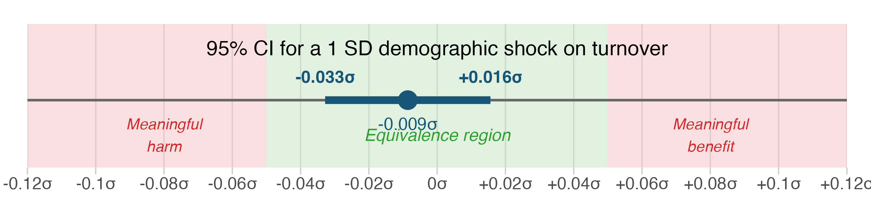
Teacher departures: bounded null

The same IV specification shows no increase in teacher exits when the buffer compresses. TOST equivalence test confirms the effect is negligibly small. Reorganisation does not trigger turnover.

PERSAL teacher-level personnel records. Outcome: proportion of educators departing to other schools. IV: k=10 LOO demographic instrument.

TALK: The second concern: if you compress the buffer, teachers will leave. The data reject this. When the demographic shock forces the buffer to compress, teacher departures do not increase — it is a precise zero, bounded by equivalence testing. Why? Because South African public-school teachers earn a substantial wage premium. Their exit options are limited. The buffer persists not because removing it would cause turnover, but because reorganising class schedules is hard work and principals face no accountability for not doing it.

Having shown that forced reorganisation improves efficiency without harming learning, we now test whether it triggers teacher exit.

• Dependent variable: Proportion of educators departing the school (from PERSAL records).
• Instrument: The same LOO demographic shock.
• Test: TOST equivalence test with bounds at ±δ.

But Don’t Teachers Need Free Periods to Prepare?

Component	Description	Hours
Formal school day	Mandated on-site time (PAM requirement)	7.0 h
Instructional periods	~6 periods × 45 min	4.5 h
Breaks	Recess + lunch (rest, not prep)	1.0 h
Within-day non-contact	Admin, assembly, non-instructional tasks	1.5 h
Informal school day	~400 h/year mandated for planning and marking	~2.0 h/day

Even at TCR = 1.0 (every teacher teaching every period), teachers have ~3.5 hours daily for preparation
(1.5 h within-day non-contact + 2 h mandated informal time).

The current TCR of 1.22 gives additional free periods during instruction — beyond what is already ample.

TALK: Don’t teachers need those free periods? No — or at least, not as many. The PAM requires 7 hours on-site. About 4.5 are instructional. Breaks are 1 hour. The remaining 1.5 hours within the day are non-instructional. On top of that, 400 hours per year — about 2 hours per day — are mandated for planning and marking. Even at TCR = 1.0, teachers would have 3.5 hours daily for preparation. The current TCR of 1.22 gives additional free periods on top of already-ample preparation time.

PART V: SO WHAT?

Scale, Context, and Why This Isn’t Just South Africa

R22.3 billion per year

That is 18.2% of instructional time purchased as teacher leisure, not smaller classes.

This exceeds the combined spending on the school feeding programme and all textbooks.

Programme	Annual spend
School Nutrition Programme	R9.1bn
Learning & Teaching Materials	R6.8bn
Non-contact buffer	R22.3bn

Not Just South Africa

Tanzania: 2.5 teachers per class, yet class sizes exceed 80.

The extensive-margin failure — teachers employed but not deployed — is unmeasured in most developing countries.

The World Bank tracks whether teachers are present. It does not track whether they are deployed.

🔍 International TCR comparison: B15

TALK: R22.3 billion per year — more than the combined spending on school nutrition and all learning materials. And this is not money that has gone missing. It is purchasing free periods instead of instruction. Redeploying it requires no additional fiscal appropriation, only better management. And this is not just South Africa — the pattern repeats across the developing world wherever we measure it.

Policy Implications

1. You cannot hire your way to smaller classes.

Without changing deployment norms, additional teachers expand the buffer rather than shrinking classes. The standard policy lever (more hiring) is pouring water into a leaky bucket.

2. Enforce existing contact-time rules.

National policy already mandates 85% contact time. The average is 82%. This is a monitoring problem, not a resource problem.

3. Mandate periodic class schedule reviews.

If the binding constraint is path-dependence, a mandated review of class structures every few years replicates the “forcing event” that the demographic shock provides naturally. Require principals to justify their configuration against an efficient benchmark.

TALK: Three implications. First, you cannot hire your way to smaller classes — new hires expand the buffer. Second, enforce existing rules — 85 per cent contact time is already mandated. Third, mandate periodic class schedule reviews. My results show that external pressure forces improvement. A mandated review replicates that forcing event.

By opening the black box of school HR, I solve the puzzle of why hiring more teachers fails to shrink classes.

The public sector does not have a capacity problem. It has an incentive problem.

When pushed, the state can deliver. It just prefers not to.

TALK: By opening the black box of school HR, we solve the puzzle of why input-based spending fails to reduce class sizes. The answer is not that the public sector lacks capacity — 19 per cent of instructional time sits idle. The answer is that it lacks the incentive to use it. When pushed, the state can deliver. It just prefers not to. Thank you.

Appendix Slides

B1: The Optimisation Problem (Formal)

← Back to Main Slide | ← Back to Main Slide

\[\min_{\{a_{tg}\}} \;\; \text{ECS}_i \;=\; \frac{1}{N_i} \sum_{g} \sum_{c \in g} n_{gc}^2 / n_g\]

subject to:

\[\sum_{g} a_{tg} \leq H_t \quad \forall\, t \quad \text{(teacher time constraint)}\]

\[\sum_{t} a_{tg} \geq C_g \quad \forall\, g \quad \text{(class coverage constraint)}\]

\[a_{tg} \in \{0, 1, \ldots\} \quad \text{(integer assignment)}\]

The constrained optimisation holds teacher headcount fixed and finds the class-size-minimising assignment of teachers to grades. Scenarios S1–S4 correspond to sequential relaxation of constraints.

Full derivation and constraint definitions in the paper, Section 3.

B2: Anderson-Rubin Confidence Set

← Back to Main Slide

Statistic	Value
AR 95% Confidence Interval	[−0.576, −0.029]
AR Chi-squared statistic	5.41
AR p-value	0.020
Interpretation	Excludes zero; result robust to arbitrarily weak instruments

The Anderson-Rubin test inverts the Wald statistic to construct a confidence set that is valid regardless of instrument strength. The interval excludes zero, confirming the 2SLS result.

B3: Effective F-Statistic (Montiel-Olea-Pflueger)

← Back to Main Slide

Diagnostic	Value	Critical value	Verdict
Montiel-Olea-Pflueger F	39.8	23.1 (5% worst-case bias)	PASS
Cragg-Donald F	42.1	16.4 (Stock-Yogo 10% size)	PASS
Kleibergen-Paap F	38.5	—	Robust to heteroskedasticity

MOP is the appropriate diagnostic for heteroskedastic data. All three diagnostics confirm instrument strength.

B4: Power-Exogeneity Frontier

← Back to Main Slide

Neighbours (k)	2SLS coefficient	Effective F	AR 95% CI
5	−0.31	18.2	[−0.82, −0.01]
10	−0.27	39.8	[−0.58, −0.03]
15	−0.25	51.4	[−0.47, −0.05]
20	−0.24	58.7	[−0.43, −0.06]
30	−0.22	63.1	[−0.39, −0.07]
50	−0.19	64.8	[−0.35, −0.05]

Increasing k trades LOO exogeneity for first-stage power. The coefficient attenuates gradually, consistent with increasing bias from own-school contamination. k=10 balances power and exogeneity.

B5: Event Study Plot (Levels-Based)

← Back to Main Slide

Pre-trend coefficients are indistinguishable from zero. The shock hits contemporaneously and dissipates within one year. Monte Carlo simulations confirm correct size (5.2% rejection rate at nominal 5%).

Event study with 3 leads and 3 lags. 95% CIs from school-clustered SEs. N ≈ 14,600 school-year observations.

B6: Conley Spatial Standard Errors

← Back to Main Slide | ← Back to Main Slide

SE type	Coefficient	SE	95% CI	Significant?
Clustered (school)	−0.270	0.098	[−0.462, −0.078]	Yes
Conley 25 km	−0.270	0.112	[−0.490, −0.050]	Yes
Conley 50 km	−0.270	0.119	[−0.503, −0.037]	Yes
Conley 100 km	−0.270	0.127	[−0.519, −0.021]	Yes

All significance levels preserved under spatial dependence at every cutoff. The result is not driven by spatial clustering.

B7: Leave-One-Out School Robustness

← Back to Main Slide

[Figure: outputs/01_figures/loo_school_robustness_histogram.svg]

Histogram of re-estimated 2SLS coefficients, each dropping one school from the sample. Distribution centred at −0.270 with narrow spread. The most influential school shifts the coefficient by less than 0.008. No single school drives the result.

B8: Placebo Outcomes

← Back to Main Slide | ← Back to Main Slide

Placebo outcome	Coefficient	SE	p-value	Verdict
Change in teachers	0.003	0.018	0.87	Null
Change in STR	−0.01	0.04	0.82	Null
Change in school quintile	0.000	0.002	0.94	Null
Change in fee status	0.001	0.003	0.71	Null

The instrument does not predict changes in teacher numbers, school wealth quintile, or fee status. It operates exclusively through grade composition, as intended.

B9: Retention and Migration Channel

← Back to Main Slide

Instrument	Predicts retention?	Predicts grade composition?
Own-school demographics	Yes (p < 0.01)	Yes
k=10 LOO demographics	No (p = 0.43)	Yes

Own-school demographics predict retention because principals’ retention decisions respond to their own enrolment. The LOO instrument eliminates this channel. Worst-case bias from residual retention contamination: 7.5% of the reduced form estimate.

B10: Hausman Comparison Across Instruments

← Back to Main Slide

Instrument	2SLS coefficient	SE	Hausman test vs. k=10
k=5 LOO	−0.31	0.14	p = 0.78
k=10 LOO	−0.27	0.10	—
Circuit LOO	−0.24	0.11	p = 0.82

Fail to reject equality across all instrument definitions. The coefficient is stable across neighbourhood definitions, consistent with a common underlying causal parameter.

B11: Conley Sensitivity (Direct Effect Bound)

← Back to Main Slide

How large would a direct instrument effect on efficiency need to be to overturn the result?

Answer: 9.3% of the reduced form.

A direct effect this large would imply that neighbourhood demographics affect school organisation through channels entirely unrelated to grade composition — a difficult story to tell given the balance checks.

Following Conley, Hansen, and Rossi (2012). The exclusion restriction can be substantially violated before the sign of the result changes.

B12: Balance Table

← Back to Main Slide

School observable	Coefficient on Z	SE	p-value
Wealth quintile	0.002	0.014	0.89
Fee status	−0.001	0.008	0.91
Baseline enrolment	1.23	3.41	0.72
Urban indicator	0.003	0.011	0.78
Baseline STR	−0.02	0.09	0.83

Joint F-test: F(5, 6285) = 0.31, p = 0.91

The instrument is uncorrelated with all observable school characteristics. The demographic shock is as good as randomly assigned conditional on controls.

B13: Data Sources

← Back to Main Slide

Dataset	Content	Records	Years	Cross-validation
LURITS	Learner-to-class assignment records	5.4m per year	2022–2024	Matched to EMIS at 99.2%
EMIS	School infrastructure, staffing, classes	6,291 schools	2018–2024	Annual census
PERSAL	Teacher-level personnel records	~240k educators	2018–2024	Matched to EMIS at 97.8%

All three datasets are administrative records maintained by the Department of Basic Education and linked at the school level. LURITS provides the individual learner-to-class mappings that enable class schedule reconstruction.

B14: Learning Outcomes — Full Results

← Back to Main Slide

Outcome	OLS	IV (2SLS)	TOST equiv. bound
Math value-added (SD)	0.002 (0.009)	0.006 (0.025)	[−0.041, 0.060]
Reading value-added (SD)	−0.001 (0.010)	0.011 (0.028)	[−0.038, 0.067]
Composite value-added (SD)	0.001 (0.008)	0.008 (0.024)	[−0.036, 0.058]

All point estimates are near zero. TOST equivalence bounds confirm that the entire 95% CI falls within the ±0.10 SD negligibility threshold. Standard errors in parentheses, school-clustered.

B15: International Teachers-per-Class Comparison

← Back to Main Slide

Country	Teachers per class	Mean class size	STR
South Africa	1.22	43.3	32.5
Tanzania	2.50	82.0	45.0
Kenya	1.35	52.0	40.0
India (UP)	1.60	55.0	35.0
OECD average	~1.2	21.0	14.0

Note on OECD: The OECD average TCR of ~1.2 reflects a very different composition — specialist teachers, special education staff, and small-group instruction — rather than managerial slack. OECD STR of 14 includes non-classroom teaching staff. Direct cross-country TCR comparisons require careful definitional alignment.

A teachers-per-class ratio above 1.0 indicates reserve capacity. The phenomenon is widespread across developing countries but unmeasured in most contexts. South Africa’s administrative data enable the first precise decomposition.

South Africa: author’s calculations. Tanzania, Kenya, India: World Bank SDI reports and administrative data estimates. OECD: Education at a Glance 2023 (classroom teaching staff, primary level).